GLSL Path Tracing

In Light and Rendering I looked at the physics of how light interacts with matter, and in Volume Rendering, Path Tracing edition I covered how to trace that light through a participating medium with a Monte Carlo approach. This time the subject isn’t a medium but a surface. We’ll fire light at a scene defined by an SDF, follow each ray as it reflects and diffuses off surfaces, and build up a single image — taking a GLSL path tracer apart from start to finish.

The rendering equation

Physically based rendering ultimately comes down to solving one equation. The rendering equation, formalized by James Kajiya in his legendary 1986 paper The Rendering Equation, is as follows.

The light $L_o$ leaving a point $\mathbf{p}$ in direction $\omega_o$ is the sum of the light $L_e$ the point emits on its own and the light $L_i$ arriving from every direction $\omega_i$ over the hemisphere $\Omega$, reflected off the surface. $f_r$ is the BRDF (Bidirectional Reflectance Distribution Function), which defines the relationship between the incoming and outgoing directions, and $(\omega_i \cdot \mathbf{n})$ is the Lambert cosine term, which accounts for light glancing in at an angle contributing less to the surface.

The problem is that the right-hand side contains the same integral again, hidden inside $L_i$. The light arriving at a point is light that left another surface, which is light that came from yet another surface. There’s no way to solve this recursion in closed form.

So we use the same strategy as in the volume rendering post. Instead of integrating over the whole hemisphere, we pick one direction at random, follow the light along it, and repeat many times and average. That’s Monte Carlo integration.

Here $p(\omega_i)$ is the probability density of picking that direction. Dividing by the probability in the denominator is the crux: when a rarely-picked direction happens to be chosen, we have to scale it up accordingly so the estimate doesn’t drift to one side. The variable that accumulates this correction factor at every bounce is usually called the throughput. The whole code is essentially this one line implemented for a single ray.

Scene as distance: SDF and Ray Marching

The scene is defined not with polygons but with an SDF (Signed Distance Function) — a function that, given a point in space, returns the distance to the nearest surface. The floor is just a plane.

float sdPlane(vec3 p, vec3 n, float h)
{
    return dot(p, n) + h;
}

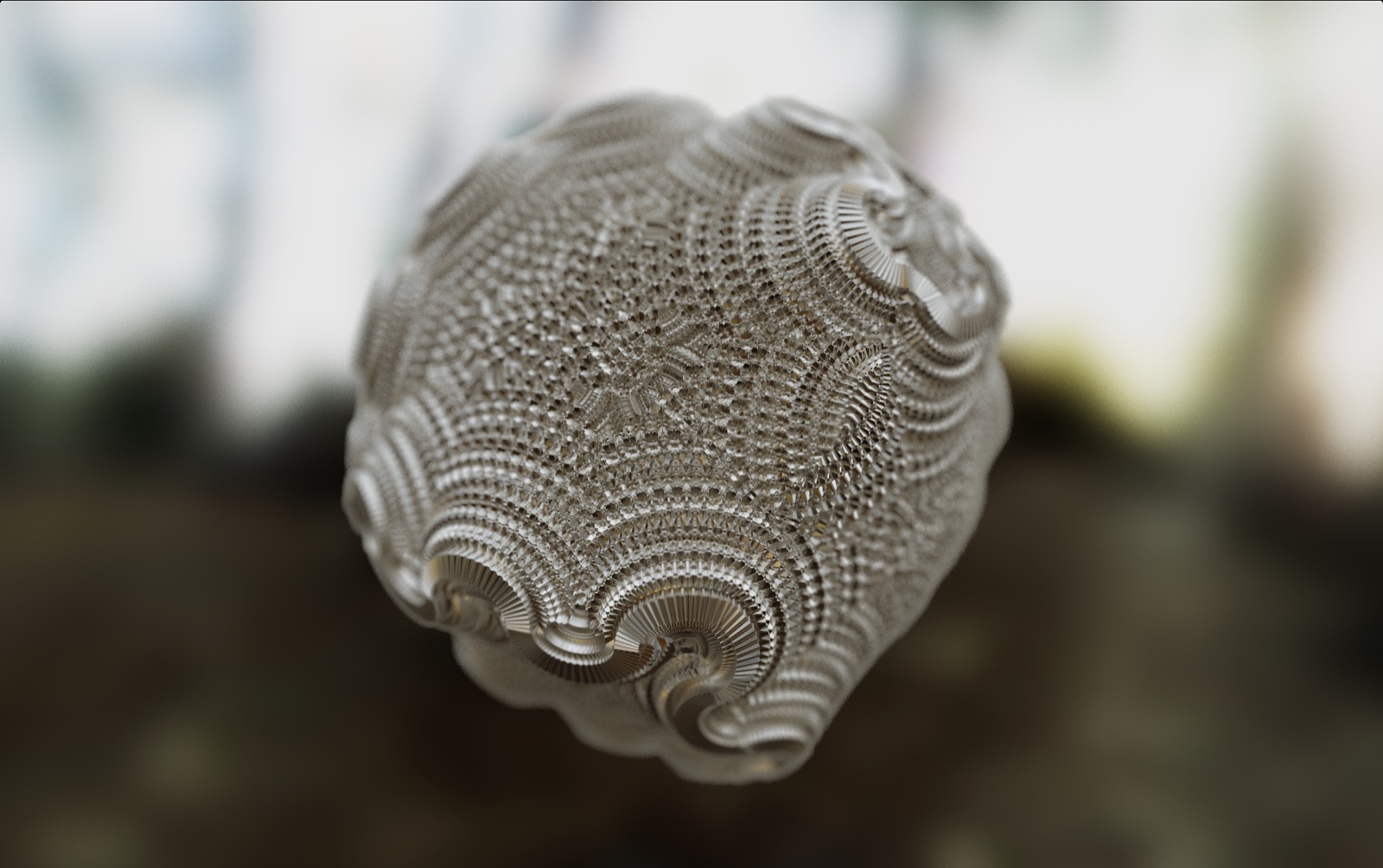
The interesting part is the star of the show, the fractal. We build a distance field by repeating a process of folding, rotating, and translating space three times.

vec2 foldPair(vec2 v)
{
    float s = v.x + v.y;
    float d = v.x - v.y;
    return 0.5 * vec2(abs(s) + d, abs(s) - d);
}

float fractal(vec3 p)
{
    for (int i = 0; i < 3; i++)
    {
        rotX(p, iTime * 0.1);
        rotY(p, iTime * 0.2);
        rotZ(p, iTime * 0.3);

        p.xy = foldPair(p.xy);
        p.yz = foldPair(p.yz);
        p.zx = foldPair(p.zx);

        p -= 0.2;
    }

    return length(p) - 0.3;
}

foldPair is an operation that folds a plane across its diagonal. The function just returns the distance field of a sphere, length(p) - 0.3, at the end — but because space was folded several times beforehand, a single sphere gets replicated as many times as it was folded, appearing as an intricate fractal shape.

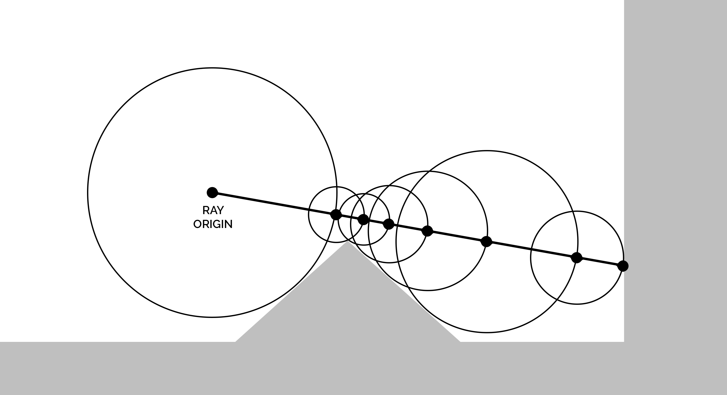
Advancing a ray along this distance field is what Ray Marching is. Since it’s guaranteed that nothing lies within the distance from the current position to the surface, we can safely jump by that distance, stepping forward until we reach the surface.

bool RayMarch(vec3 ro, vec3 rd, out vec3 hitPos, out HitInfo hit)
{
    float t = 0.0;

    for (int i = 0; i < MAX_MARCH_STEPS; i++)
    {
        vec3 p = ro + rd * t;
        hit = mapScene(p);

        if (hit.dist < SURF_EPS)
        {
            hitPos = p;
            return true;
        }

        if (t > MAX_DIST)
        {
            break;
        }

        t += max(hit.dist * 0.8, SURF_EPS);
    }

    hitPos = ro + rd * t;
    return false;
}

A distance field built by folding space can sometimes overestimate the true distance, so jumping by the full amount risks tunneling through the surface. That’s why we advance cautiously by only 80% of the distance (hit.dist * 0.8).

Thin lens camera

The simplest camera fires rays from a single point (a pinhole). Everything then comes out sharp, but it can’t reproduce the depth of field our eyes or a real lens create. So we use a thin lens model.

vec3 pinholeDir = normalize(
    forward * focalLength +
    right * screen.x +
    up * screen.y
);

float focusDist = 1.4;
float lensRadius = 0.05;

vec3 focusPoint = camPos + pinholeDir * focusDist;

vec2 lens = RandomInDisk(rngState) * lensRadius;

vec3 ro = camPos + right * lens.x + up * lens.y;
vec3 rd = normalize(focusPoint - ro);

Here’s the idea. First, along the direction a ray would have gone in a pinhole camera (pinholeDir), we place a point on the focal plane (focusPoint) at the focus distance (focusDist). Then we scatter the ray’s origin not to a single point but to a random point on a disk of radius lensRadius (RandomInDisk). The origin jitters, but since every ray aims at the same focusPoint, objects on the focal plane always converge to a point and stay sharp, while objects nearer or farther scatter and blur. Increasing lensRadius strengthens the blur, like opening up the aperture.

Following the ray

Now the main body: the path tracing loop. A single ray bounces up to MAX_BOUNCES times through the scene, gathering light.

vec3 radiance = vec3(0.0);
vec3 throughput = vec3(1.0);

for (int bounce = 0; bounce < MAX_BOUNCES; bounce++)
{
    vec3 hitPos;
    HitInfo hit;

    bool didHit = RayMarch(ro, rd, hitPos, hit);

    if (!didHit)
    {
        radiance += throughput * SampleEnvironment(rd);
        break;
    }

    vec3 n = getNormal(hitPos);

    if (dot(n, rd) > 0.0)
    {
        n = -n;
    }

    Material mat = hit.mat;

    radiance += throughput * mat.emission;

    ro = hitPos + n * SURF_EPS * 4.0;

radiance is the light gathered so far, and throughput is the running product of the correction factor described earlier. If a ray hits nothing and escapes the scene, we sample the environment map, add that light scaled by throughput, and finish. In the end, in this path tracer all light comes entirely from the environment.

When a ray hits a surface, we first compute the normal vector. In a distance field the normal vector is obtained by taking the gradient of the distance along each axis.

vec3 getNormal(vec3 p)
{
    vec2 e = vec2(NORMAL_EPS, 0.0);

    return normalize(vec3(
        sdf(p + e.xyy) - sdf(p - e.xyy),
        sdf(p + e.yxy) - sdf(p - e.yxy),
        sdf(p + e.yyx) - sdf(p - e.yyx)
    ));
}

If the normal vector faces the same way as the ray, we flip it so it always faces the ray (dot(n, rd) > 0.0), and if the surface emits light on its own we add that emission. Finally we nudge the next ray’s origin slightly off the surface along the normal vector. Without this, the new ray would immediately hit the surface it just struck — a self-intersection.

Fresnel and materials

What decides whether the light hitting a surface reflects or diffuses is the material. As covered in Light and Rendering, how much light reflects at a boundary is set by the index of refraction (IOR), and that ratio changes with viewing angle. The reflectance $F_0$ when viewed head-on is as follows.

float F0FromIOR(float n1, float n2)
{
    float r0 = (n1 - n2) / (n1 + n2);
    return r0 * r0;
}

Computing the angular variation exactly every time is expensive, so we usually use the Schlick approximation.

The more grazing the angle at which you view the surface ($\cos\theta \to 0$), the closer the reflectance gets to 1. This is why, looking at a puddle head-on you see the bottom, but viewed at a shallow angle from far away the sky reflects in it like a mirror.

float cosTheta = clamp(dot(n, -rd), 0.0, 1.0);

float dielectricF0 = F0FromIOR(1.0, mat.ior);
vec3 F0 = mix(vec3(dielectricF0), mat.albedo, mat.metallic);

float x = clamp(1.0 - cosTheta, 0.0, 1.0);
vec3 F = F0 + (1.0 - F0) * x * x * x * x * x;

Here you can see the common trick of unifying metal and non-metal into a single formula. A non-metal (dielectric) gives a weak, grayish reflection ($F_0 \approx 0.04$), and its color comes from diffuse. A metal, on the other hand, has no diffuse, and the reflection color itself is the metal’s color. So we use the metallic value to mix $F_0$ between the dielectric value and the object’s own color (albedo), tinting the reflection more the more metallic it is.

Reflect or diffuse: a probabilistic choice

Every time light bounces, it splits into two paths: specular and diffuse. Tracing both makes the rays double at every bounce and explode. So we pick only one of them probabilistically.

vec3 specularWeight = F;
vec3 diffuseWeight = mat.albedo * (1.0 - mat.metallic) * (1.0 - F);

float specularProb = max(specularWeight.r, max(specularWeight.g, specularWeight.b));
specularProb = clamp(specularProb, 0.0, 1.0);

bool chooseSpecular = RandomFloat01(rngState) < specularProb;

We set the probability of going specular proportional to the Fresnel reflectance $F$. The more grazing the surface, the larger $F$, so we naturally pick the specular side more often. Picking important directions more frequently like this is importance sampling, and it’s the secret to getting a less noisy image with fewer samples.

if (chooseSpecular)
{
    vec3 reflected = reflect(rd, n);

    float a = mat.roughness * mat.roughness;

    rd = normalize(mix(
        reflected,
        RandomCosineHemisphere(reflected, rngState),
        a
    ));

    throughput *= specularWeight / max(specularProb, 1e-4);
}
else
{
    rd = RandomCosineHemisphere(n, rngState);

    throughput *= diffuseWeight / max(1.0 - specularProb, 1e-4);
}

If specular is chosen, we take the perfect mirror direction (reflect) as the basis and scatter the direction according to roughness. At roughness 0 it’s a pure mirror; near 1 it becomes a glossy surface that spreads widely around the reflection direction. It’s not a proper microfacet-based model like GGX — just a lightweight approximation that linearly interpolates between the specular direction and a cosine distribution — but it produces a convincing gloss at low cost.

If diffuse is chosen, we draw a direction from a cosine-weighted hemisphere around the normal vector. Because a Lambert surface follows exactly this distribution, the $\cos\theta$ term and the probability $p(\omega_i)$ in the Monte Carlo formula from earlier cancel out cleanly.

In both cases we multiply throughput by each path’s weight and divide by the probability with which we chose that path. Since we chose specular with probability specularProb, we divide by specularProb, and diffuse by 1 - specularProb. This division is what makes the result unbiased — on average the same as tracing both — even though we only trace one of them.

Russian Roulette

After bouncing several times, a ray’s throughput shrinks until it barely contributes to the final image. Tracing it to the bitter end anyway is wasteful, but cutting it off at a fixed count loses that much light and darkens the image. The compromise between the two is Russian Roulette.

if (bounce > 1)
{
    float p = max(throughput.r, max(throughput.g, throughput.b));
    p = clamp(p, 0.05, 0.95);

    if (RandomFloat01(rngState) > p)
    {
        break;
    }

    throughput /= p;
}

The smaller the throughput, the higher the probability we kill the ray. But surviving rays are scaled back up by throughput /= p. Because of this correction the expected value stays the same, so cutting rays off midway introduces no bias into the result. Computation drops while brightness is preserved.

Progressive accumulation

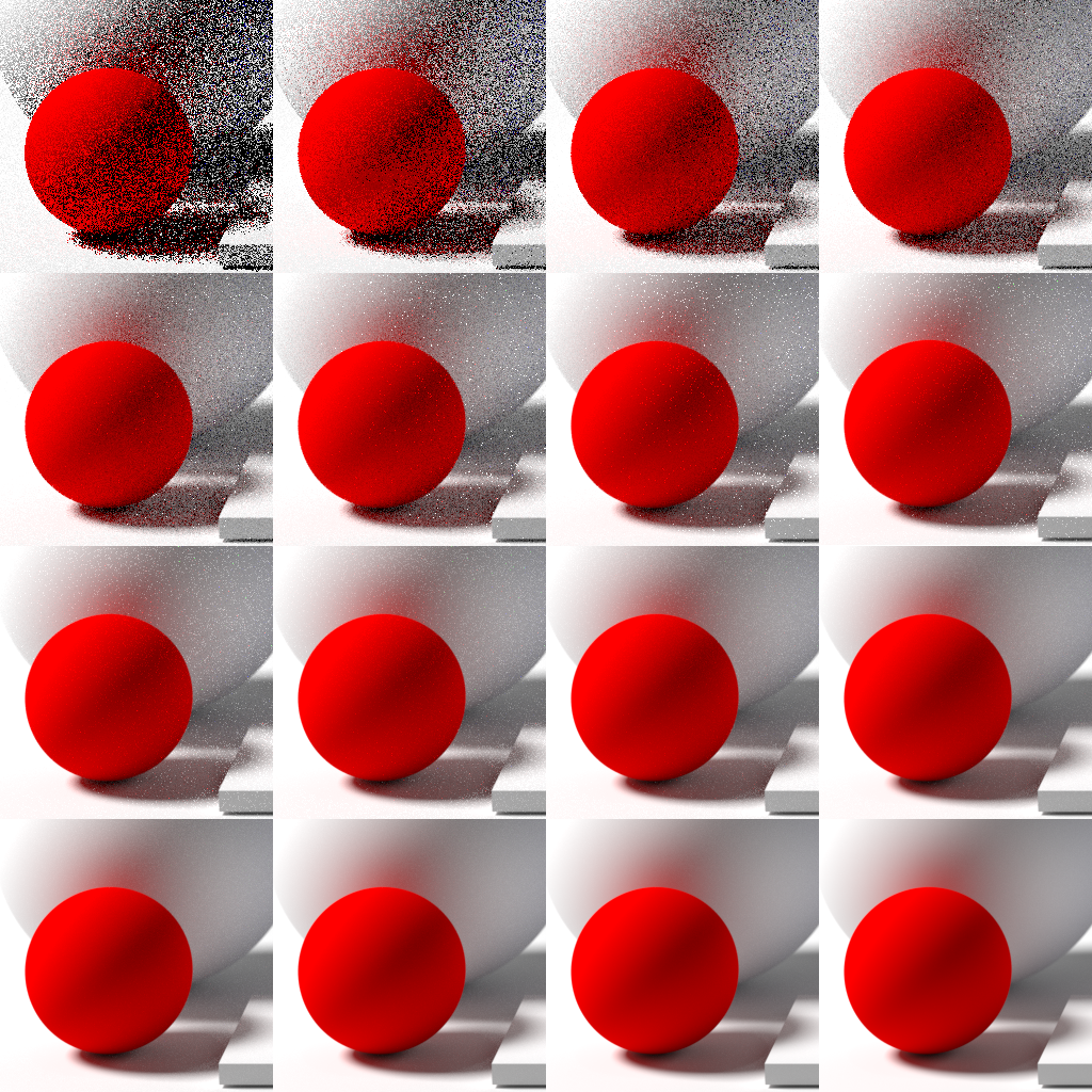
The result of a single ray, a single frame, is a lump of noise. Path tracing inherently needs the average of many samples. So each frame we blend the result with the previous frame and accumulate.

vec3 previous = texture(iChannel0, uv).rgb;

vec3 col;
if (iFrame == 0)
{
    col = radiance;
}
else
{
    col = mix(previous, radiance, 0.05);
}

Try it yourself

The full code we’ve dissected here is up on Shadertoy. You can watch the accumulation process in real time as frames pile up and the noise fades.

Wrapping up

Once you go around the code once, the skeleton of path tracing is laid bare. Fire light backwards (from camera into the scene); at each surface hit, split into specular/diffuse probabilistically with Fresnel and follow just one direction; multiply along the throughput corrected by the probability of that choice; and finish by either picking up light from the environment map or terminating with Russian Roulette. Then stack the noisy results across frames and average them.

The physics from Light and Rendering becomes code, line by line, inside this shader. Approximating the rendering equation — which can’t be solved in closed form — with Monte Carlo sampling and a running average is the heart of path tracing.